Geographic Variation in Life-History Traits of Black Sea Bass (Centropristis striata) During a Rapid Range Expansion

Introduction

Climate-induced range shifts have become common in recent decades. Species are altering their distributions to avoid climatic stress, which is modifying the structure and function of ecosystems globally (e.g., Parmesan and Yohe, 2003; Perry et al., 2005; Poloczanska et al., 2013; Pecl et al., 2017). This movement is expected to intensify, and may already be occurring at unprecedented rates (Lawing and Polly, 2011; Pecl et al., 2017). As species undergo range shifts, they encounter unique selective pressures that may alter life-history traits and lead to increased spatial heterogeneity among populations (Burton et al., 2010; Phillips et al., 2010). These shifts can greatly complicate conservation and management efforts, particularly if the impact of range expansion on a species’ population dynamics is not well understood.

Geographic variation in life-history traits often arises in response to different environmental and demographic gradients experienced across the range of a species (e.g., Roff, 1993; Brown, 1995). For instance, populations not constrained by density-dependent effects often invest less in competitive (K) and more in reproductive (r) capabilities (Charlesworth, 1971; Roughgarden, 1971). In contrast, populations that are density-dependent are often K-selected because successful propagation is related to fitness in high density areas (Charlesworth, 1971; Roughgarden, 1971). Although the “abundant center” distribution does not always occur in natural populations (e.g., Sagarin and Gaines, 2002), range expanding species are expected to exhibit lower population density along the expanding range edge in comparison to more centralized populations (Burton et al., 2010; Phillips et al., 2010). Environmental heterogeneity across a species’ range can also drive life-history variation (Brander, 2010). In particular, temperature and the length of the growing season can strongly influence growth and the timing of maturation in fish (Pauly, 1980; Conover, 1990; Pörtner et al., 2001). Spatial variations in predation pressure (e.g., Reznick et al., 1990; Benard, 2004), harvesting (e.g., Jorgensen et al., 2007) and prey availability (e.g., Sherwood et al., 2007) also can influence life-history traits in fish. Collectively, these environmental and biotic processes that mediate the biology of fish species also help determine the amount of biomass that can be sustainably harvested.

Recently, emphasis has been placed on incorporating spatial heterogeneity into marine fisheries management (Ciannelli et al., 2008; Cadrin and Secor, 2009; Pascoe et al., 2009; Lorenzen et al., 2010). Traditionally, stock populations have been managed over large geographic areas where demographic and environmental variables were considered homogenous (Ciannelli et al., 2008). Spatial heterogeneity has largely been ignored due to the substantial complexity it adds to stock assessment models (Pascoe et al., 2009). However, demographic and environmental conditions are rarely homogenous throughout a species’ range, and ignoring this heterogeneity may lead to a misunderstanding of the mechanisms regulating population dynamics (Ciannelli et al., 2008; Lorenzen et al., 2010) and subsequent mismatches between harvest levels and stock productivity. Incorporating spatial heterogeneity may be of particular importance for range expanding species that can undergo rapid evolution of life-history traits (Burton et al., 2010). Yet, a big impediment to adaptively managing range shifts is that there often is little information about these species at the leading edge of their newly expanded distributions.

The black sea bass, Centropristis striata, is a temperate serranid that is distributed from the Gulf of Mexico to the Gulf of Maine (GOM) (Drohan et al., 2007). Within that range, they are managed as three separate stocks: Gulf of Mexico, Southeast U.S. Continental Shelf and Northeast U.S. Continental Shelf. The Northeast U.S. Continental Shelf stock is further defined as two sub-units, north and south of Hudson Canyon. The Northeast U.S. stock undergoes seasonal migrations, and inhabits the outer continental shelf in the winter vs. nearshore habitat in the spring and summer when spawning occurs (Moser and Shepherd, 2009). They support important commercial and recreational fisheries throughout their range.

Historically, the Northeast U.S. stock ranged from Cape Hatteras, NC to Cape Cod, MA, but in recent years the center of stock biomass has shifted poleward (Bell et al., 2015) and sea bass populations have expanded into the GOM. Very little is known about the population dynamics of sea bass in the GOM. Current stock designations are based on differences in seasonal migrations and life-history traits of sea bass south of Cape Cod, yet it is unclear if the biological characteristics of sea bass in the GOM differ from those of populations farther south. Furthermore, sea bass fisheries have recently developed in the northern GOM outside of stock assessment areas, potentially making this population vulnerable to rapid depletion (Link et al., 2011).

Sea bass are protogynous hermaphrodites (i.e., they are typically born female and transition to male as they increase in size and age), which can complicate management, particularly if accurate information on sex ratios and the mean size at which individuals change sex is not available (Alonzo et al., 2008; Provost and Jensen, 2015). Furthermore, latitudinal variation in growth rates and age-at-maturity has been observed in both the Northeast U.S. (Kolek, 1990; Caruso, 1995) and Southeast U.S. sea bass stocks (McGovern et al., 2002). Kolek (1990) and Caruso (1995) found that sea bass collected in southern Massachusetts grew faster than sea bass from New York and Virginia and Caruso (1995) also noted that sea bass collected from this area were predominantly mature. In addition, McCartney et al. (2013) observed genetic variation across a latitudinal gradient in the northern stock. These studies provide evidence that life-history variation exists within the northern stock, and further emphasize the need to understand how the northern range expansion is influencing population dynamics and structure.

The purpose of this study was to document life-history traits of sea bass collected from southern Massachusetts (i.e., native range) and two regions within the GOM (i.e., newly expanded range). We analyzed diet, growth, condition, and reproduction within these regions, and examined spatial variation that may have implications for stock assessment and management. This study represents one of the first documentations of black sea bass life-history traits at the northern extent of their newly expanded range.

Materials and Methods

Sampling Design

To determine if life-history traits of black sea bass differed between native and newly expanded populations, we collected samples from three regions: southern Massachusetts (SMA) (historic northern range limit delineated by Cape Cod), northern Massachusetts (NMA) (newly expanded range north of Cape Cod) and midcoast Maine (ME) (expanding range edge), between May and October from 2013 to 2016 (Figure 1). In SMA, fish were collected by the Massachusetts Division of Marine Fisheries trawl and trap surveys, as well as by commercial lobstermen who caught sea bass as bycatch in their lobster traps. State and federal trap and trawl surveys rarely find sea bass in NMA, so fish were also collected via hook and line by recreational fishers, as well as bycatch from lobster traps. Collecting fish caught as bycatch in lobster traps was the only successful method in Maine. Recreational and commercial sea bass fishing does not occur in this area, and state and federal trawl surveys do not encounter sea bass. Therefore, the only capture method that was the same across regions was bycatch from lobster traps. Black sea bass smaller than 10 cm total length are not commonly captured in lobster traps, but are captured by trawl surveys, so to avoid biased size estimates between capture types, we did not collect sea bass smaller than 10 cm.

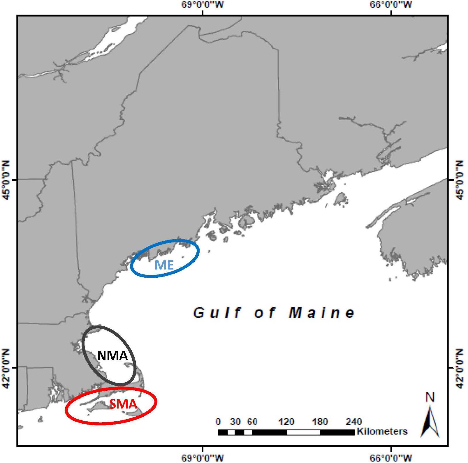
Figure 1. Map of the Gulf of Maine with field sites delineated: Maine (ME) in blue, northern Massachusetts (NMA) in gray, and southern Massachusetts (SMA) in red.

The date, location, and capture method were recorded at each site where fish were collected. To explore the influence of season on biological metrics, samples were categorized into seasons defined as spring (May–June), summer (July–August), and fall (September–October). Fish were frozen immediately after capture and transported to the laboratory where they were kept frozen until they were processed. The total length (cm), standard length (cm) and total weight (g) were measured for each fish prior to removing vital organs. Weight was also recorded after the removal of vital organs to obtain the gutted weight (g). The gonads and liver were then weighed individually, and stomachs were retained for stomach content analysis. Sagittal otoliths were removed to determine age and calculate growth rates. Small core subsections (∼1 g) were taken from muscle tissue samples to conduct stable isotope analysis to examine the diet of black sea bass.

Size Distribution and Growth

Size-frequency histograms were used to explore regional differences in black sea bass distributions. The Kolmogorov-Smirnov (K-S) test was used to compare the cumulative size frequency distribution among regions. We also compared the cumulative size frequency distribution among capture types in SMA and NMA (only one capture type was used in ME). Age determination was conducted to compare age-at-maturity of sea bass among regions. Aging techniques were adapted from the Massachusetts Division of Marine Fisheries and Northeast Fisheries Science Center protocols for black sea bass (Robillard et al., 2011; Elzey et al., 2015), which age whole otoliths up to age five, and sectioned otoliths for ages six and up. Only six fish collected in this study were six or older, and they were collected by the Massachusetts Division of Marine Fisheries in trap or trawl surveys. The otoliths of these fish were removed prior to arriving at our lab, and were sectioned and aged at the Division of Marine Fisheries Age and Growth Laboratory. For fish ages five and under, whole sagittal otoliths were immersed in mineral oil on a black background and viewed under a microscope. The number of annuli on each otolith was counted outward from the core to estimate age. Annuli were defined as continuous dark bands with no breaks. Age was calculated based on capture date and seasonal timing of when annuli form and delineate from the otolith edge (Elzey et al., 2015).

Growth was modeled using von Bertalanffy growth function (VBGF) parameter estimates obtained from the non-linear regression function in the “FSA” package (Ogle et al., 2020) in R (R Core Team, 2017) and the following equation:

where L_t is length (cm) at age t, L_inf is the asymptotic length, k is the Brody growth coefficient and t₀ is the age at which length is 0. 95% confidence intervals were calculated by bootstrapping and extracting 2.5 and 97.5% quantiles of the parameter estimates. A VBGF curve was established for all regions combined. Separate growth curves were not established for each region due to low sample sizes of the youngest and oldest age classes in NMA and ME.

Diet

Stomach contents were used to compare the diet of sea bass among regions. Stomachs were dissected and contents were weighed, counted and identified to the lowest possible taxon. Prey items were divided into the following groups: pelagic fish (bay anchovy, butterfish, herring, etc.); demersal fish (sculpin, scup, black sea bass, etc.); squid (long-fin squid); crabs (various species); shrimp (various species); lobster; benthic invertebrates (mollusks, polychetes, amphipods, algae, etc.); and unidentified fish. Partial fullness index (PFI) of prey was calculated for each fish, and mean PFI was used to compare the relative importance of prey groups among regions. Mean PFI provides a length-standardized way to determine relative volumetric prey importance (Bowering and Lilly, 1992), and was calculated as:

where w_ij is the weight of prey i for fish j, L_j is the length of fish j and n is the total number of fish sampled.

Stable isotope ratios of nitrogen (δ¹⁵N) and carbon (δ¹³C) can be used to determine the trophic position of an organism (Zanden and Rasmussen, 1999) and the source of carbon (e.g., benthic, demersal, pelagic, etc.) in marine food webs (Owens, 1987; Fry, 1988; Sherwood and Rose, 2005), respectively. Muscle tissue samples were dried in a drying oven at 60°C for 48 h, ground to a fine powder using a mortar and pestle, and weighed and packaged in 4 × 6 mm tin capsules. Samples were sent to the Colorado Plateau Stable Isotope Laboratory (Northern Arizona University, Flagstaff, AZ, United States) for analysis. Samples were combusted to produce CO₂ and N₂, from which stable nitrogen and carbon isotope ratios were analyzed using an elemental analyzer followed by gas chromatograph separation interfaced via continuous flow to an isotope ratio mass spectrometer. Stable carbon and nitrogen ratios were expressed in delta (δ) notation and defined as parts per thousand deviations from the following standard materials: Pee Dee Belemnite for δ¹³C, and N₂ in air for δ¹⁵N. To determine the level of precision of isotope results, 8% of the samples were analyzed in duplicate.

Distinctions in the overall diet among groups were assessed using a permutational multivariate analysis of variance (PerMANOVA) using the “vegan” package in R (R Core Team, 2017). Specifically, PerMANOVA was used to test the effects of region, sex, season and their interactions on the PFI’s of each prey group. PerMANOVA requires the use of a matrix of dissimilarity indices, rather than raw response values, which we calculated prior to analysis. Gower’s index was used as the dissimilarity measure because it allows for the use of double zeroes (Gower, 1971). The multivariate dispersions of each group matrix were compared using beta diversity tests to identify potential violations of PerMANOVA assumptions.

A two-step modeling approach using GLMs was used to analyze individual prey categories, similar to Stefánsson (1996). First, the presence of prey was analyzed using generalized linear models (GLMs) with binomial error distribution and logit link functions. Second, prey category abundance (i.e., PFI ≠ 0) was analyzed using GLMs with gamma error distributions and identity link functions. A similar approach using generalized additive models has also commonly been employed in diet studies (Stefánsson and Pálsson, 1997; Santos et al., 2013; Buchheister and Latour, 2015), however, GLMs are more appropriate when utilizing multiple factors (Stefánsson, 1996; Stefánsson and Pálsson, 1997). Fixed effects in both binomial and gamma GLMs included region, sex, season, and all interactions. Capture method was also included as a fixed effect, but not as an interaction term because capture method was unequally represented across the levels of the other factors. Total length was included as a covariate when analyzing prey presence, but not abundance, since PFI is a length standardized measure. Akaike information criteria (AIC) was used to assess fit and select the most parsimonious model(s). Separate three-way ANOVAs were used to test the effect of region, season and size class on carbon and nitrogen stable isotope ratios. Size classes were categorized as 10–19 cm (juveniles), 20–29 cm (50–95% mature), 30–39 cm (reproductive adults), and 40 + cm total length (≥50% male).

Condition

The length-weight relationship was estimated for all regions combined (n = 288) using the “FSA” (Ogle et al., 2020) and “stats” packages in R and a linearized version of the following equation:

where W is the whole body weight (g), L is the total length (cm), a is the intercept of the regression and b is the regression coefficient. Linearization of this equation results in the errors being additive (as opposed to multiplicative) and stabilizes the variances about the model (Ogle, 2013), allowing for linear regression methods to be used. The linear model was calculated as:

with y = log(W), x = log(L), slope = b, and intercept = log(a).

We considered two indices of physiological condition: Fulton’s condition factor K, and liver-somatic index (LSI). K is primarily an indicator of energy reserves available for somatic growth (i.e., muscle mass), while LSI is a measure of energy reserves available for reproduction (i.e., lipid storage). A length-standardized measure of Fulton’s condition factor was calculated to determine the effects of region and season on condition (Le Cren, 1951; Froese, 2006):

where W_g is the gutted fish weight (g), L is the total length (cm), and a and b are the parameters of the length-weight relationship defined above. We also calculated Fulton’s condition factor by standardizing for season, rather than size, to examine how condition varies with size and related diet ontogeny (Sherwood et al., 2007):

where K is Fulton’s condition factor and K_avg is the average condition factor (all sizes and regions) by season. LSI was calculated as:

where W_l is the liver weight and W_g is the gutted fish weight. A seasonally adjusted value was also calculated for LSI:

where LSI_avg is the average LSI (all sizes and regions) by season (spring, summer and fall).

The standardized residuals from the least-squares regression of total length and LSI or GSI were used to account for the effect of size on LSI and GSI. K_rel, residual LSI and residual GSI were analyzed using separate two-way ANOVAs where region, season, and their interaction were included as fixed effects. Post hoc multiple comparison tests were conducted using the glht function in the “multcomp” package, which conducts simultaneous tests and computes confidence intervals for parametric models (Hothorn et al., 2008; Bretz et al., 2010). Regional differences in K_adj and LSI_adj were qualitatively explored within 2 cm size intervals.

Reproduction

Sex and reproductive maturity were determined macroscopically using techniques modeled from Wuenschel et al. (2011). Macroscopic gonad analysis was sufficient for identifying developing, spawning capable and spent stages, and therefore allowed us to classify samples as mature or immature for subsequent analyses.

The gonadosomatic index (GSI) of each fish was calculated using the following equation:

where W_g is gonad weight and W_t is total weight. The sex ratio-at-length was determined separately for males and females using a logistic regression in R (R Core Team, 2017) with the following equation:

where p is the proportion of males or females at length L, k is a slope parameter, and L₅₀ is the length at which 50% of the fish are male or female, respectively. Maturity-at-length for both sexes combined was determined using the same equation, where p is the proportion of mature fish at length L, and L₅₀ is the length at which 50% of the fish are mature. Sex ratio-at-length and maturity-at-length were calculated using all regions combined, due to the small sample size within each 1 cm size bin when regions were separated. Age-at-maturity for both sexes combined was determined for all regions combined, as well as each region separately, using a logistic regression in R (R Core Team, 2017) with the following equation:

where p is the proportion of mature fish at age A, k is a slope parameter, and A₅₀ is the age at which 50% of the fish are mature. We chose to combine sexes to determine length-at-maturity and age-at-maturity because this was the method used in the most recent black sea bass stock assessment (Northeast Fisheries Science Center [NEFSC], 2016). 95% confidence intervals were calculated for sex ratio-, maturity-, and age-at-length by bootstrapping and extracting 2.5 and 97.5% quantiles of the parameter estimates using the “FSA” package (Ogle et al., 2020) in R (R Core Team, 2017). We explored whether the proportion of males and females, as well as the proportion of mature and immature fish, differed among region using Chi-Square tests.

Results

Size Frequency and Growth

Of the 288 sea bass collected between 2013 and 2016, 131 were captured in SMA, 109 in NMA and 48 in ME. There was no significant difference in the cumulative size frequency of sea bass collected among capture types in NMA and SMA (K-S test, p > 0.05 for all comparisons). Large sea bass were significantly more frequent in NMA compared to ME and SMA (K-S test, p < 0.001 for both comparisons) and small sea bass were significantly more frequent in ME compared to SMA (K-S test, p = 0.01; Figure 2). The VBGF curve for all regions combined revealed greater length-at-age estimates than the 2016 black sea bass stock assessment, particularly for younger fish (Table 1 and Figure 3).

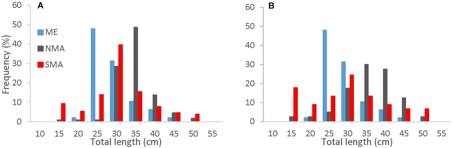
Figure 2. Cumulative length frequency distribution of black sea bass collected in Maine (blue), northern Massachusetts (gray) and southern Massachusetts (red) for (A) all capture methods combined, and (B) trap caught fish only.

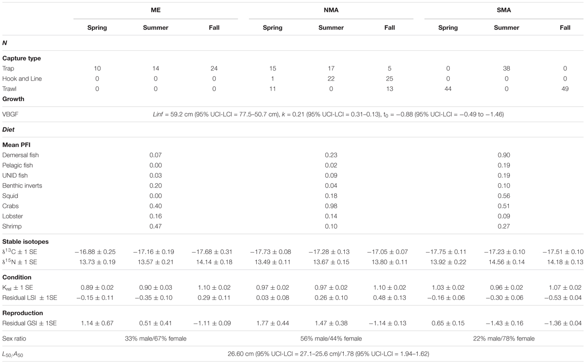
Table 1. Black sea bass sample sizes and life-history parameter estimates by region and season.

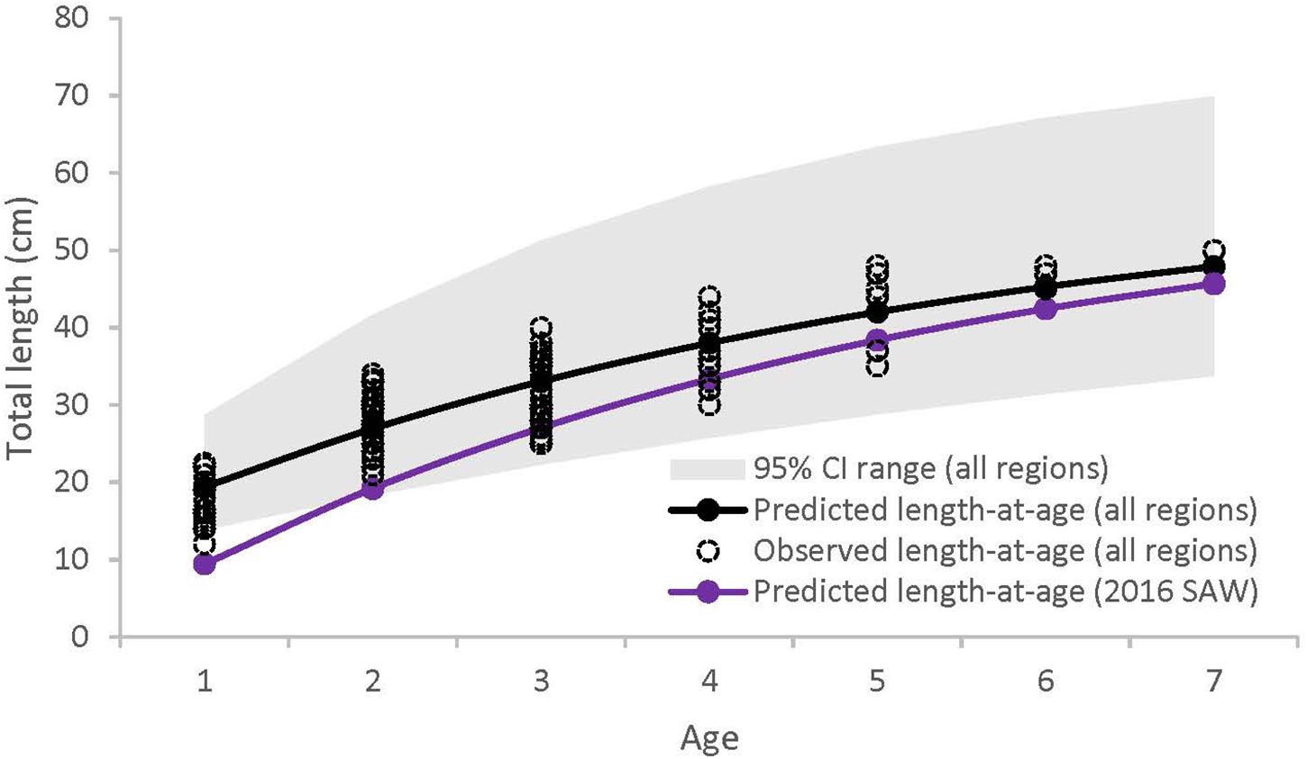
Figure 3. Von Bertalanffy growth curves for black sea bass from all regions combined (black), and from the 2016 Black Sea Bass Stock Assessment (purple) (Northeast Fisheries Science Center [NEFSC], 2016). Gray shaded area represents 95% confidence intervals for all regions combined (95% confidence intervals not available for 2016 Black Sea Bass Stock Assessment).

Diet

Sea bass diet varied among region and season, and also varied with size (Figure 4). Demersal fish, pelagic fish and squid comprised 47–66% of sea bass diet in SMA, but only 20–29% in NMA and 8% in ME. Meanwhile, crustaceans (e.g., shrimp, crabs, lobster) accounted for 31–53% of sea bass diet in SMA, 69–76% in NMA and 78% in ME (Table 1). The best fitting binomial and gamma GLMs included various combinations of explanatory variables. Region and season were typically the two most important factors in the models, emphasizing the importance of both spatial and temporal dynamics in trophic interactions. Sex did not significantly influence the presence or abundance of prey. Overall, total length and capture method did not significantly influence presence or abundance for the majority of prey groups (Supplementary Figure S1).

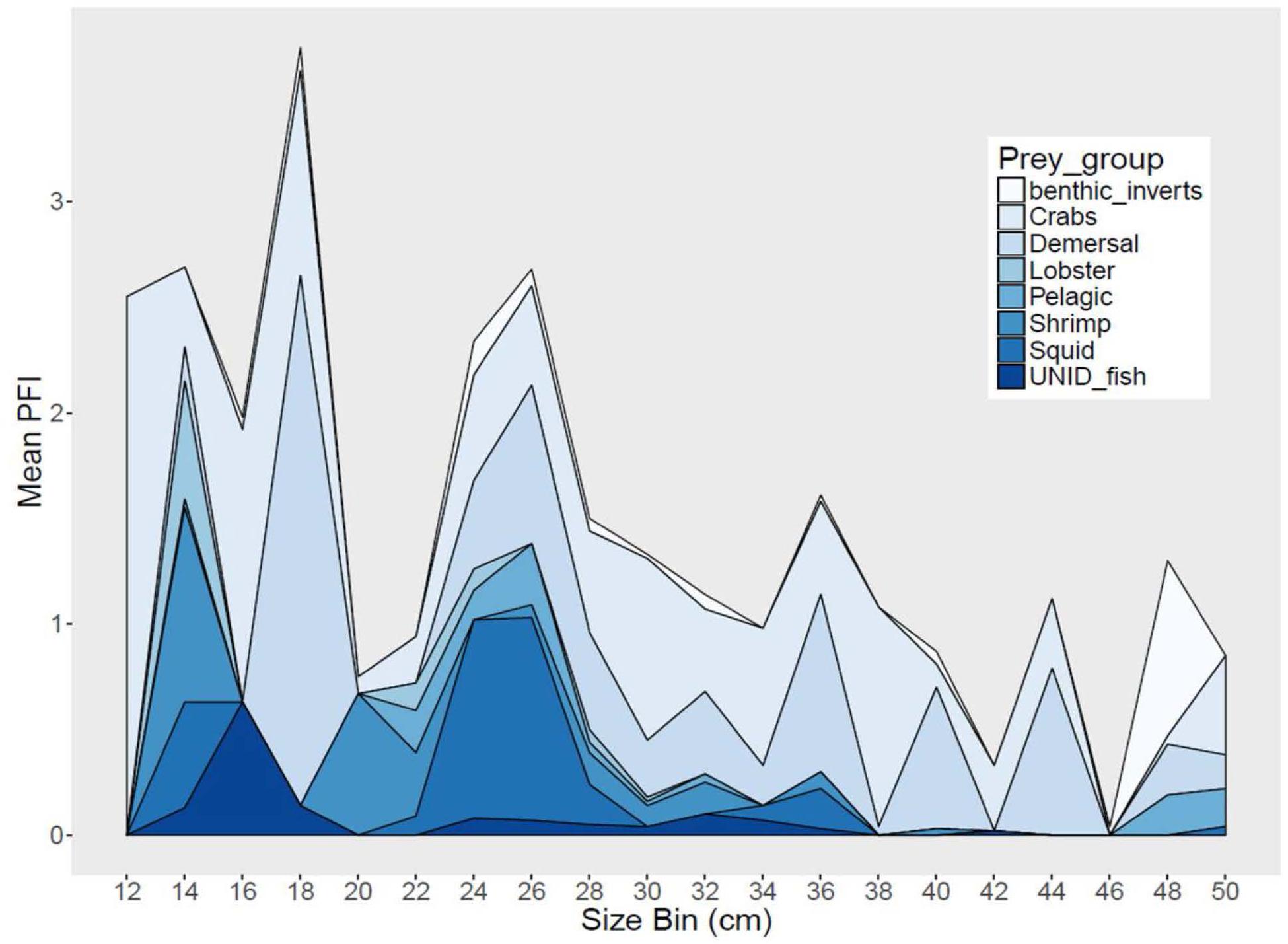
Figure 4. Stacked area graph of mean partial fullness index (Mean PFI) by 2 cm size bins for black sea bass from all regions combined.

The presence of demersal fish significantly differed by region (x² = 23.5, p < 0.001), season (x² = 39.2, p < 0.001) and total length (x² = 9.5, p = 0.002). Demersal fish were more frequent in the stomachs of SMA fish compared to NMA (Tukey’s HSD, p < 0.001) and ME (Tukey’s HSD, p = 0.01) fish, and significantly more frequent in the fall compared to the summer (Tukey’s HSD, p = 0.001). No demersal fish were found in the stomachs of fish collected in the spring. Demersal fish regularly occurred in the diet of sea bass measuring 24–40 cm total length, but were more variable in smaller and larger fish. None of the factors tested significantly influenced the abundance of demersal fish.

The presence of squid significantly differed by region (x² = 10.86, p < 0.001) and season (x² = 21.59, p < 0.001). Squid were significantly more frequent in the stomachs of fish collected in the fall compared to the summer (Tukey’s HSD, p = 0.008) and spring (Tukey’s HSD, p = 0.009), and significantly more frequent in SMA fish compared to NMA fish (Tukey’s HSD, p = 0.003). No squid were found in the diet of fish captured in ME.

There was a significant interaction between region and season (x² = 21.81, p < 0.001) on the presence of shrimp biomass in black sea bass stomachs. Shrimp were significantly more frequent in the stomachs of fish collected in SMA in the spring compared to summer (Tukey’s HSD, p = 0.012) and fall (Tukey’s HSD, p = 0.013). Similar to presence, there was an interaction between region and season on shrimp abundance (x² = 3.35, p = 0.001). Shrimp were less abundant in SMA in the fall compared to spring (Tukey’s HSD, p < 0.001) and summer (Tukey’s HSD, p < 0.001), and more abundant in the summer in SMA compared to ME (Tukey’s HSD, p = 0.03).

The presence of crabs significantly differed by region (x² = 29.70, p < 0.001) and season (x² = 26.64, p < 0.001) independently. Crabs were significantly more frequent in the stomachs of fish collected in NMA compared to ME (Tukey’s HSD, p < 0.001) and in the fall compared to the spring (Tukey’s HSD, p < 0.001). The abundance of crabs significantly differed by capture method (x² = 9.35, p = 0.012). There was a significantly greater abundance of crabs in the stomachs of hook and line caught fish compared to trap (Tukey’s HSD, p = 0.022) and trawl (Tukey’s HSD, p = 0.05) caught fish.

The consumption of benthic invertebrates (e.g., mollusks, polychetes, tunicates) significantly differed by region (x² = 14.15, p < 0.001) and season (x² = 34.99, p < 0.001). The presence of benthic inverts was significantly greater in SMA compared to ME (Tukey’s HSD, p = 0.012), and significantly lower in the summer compared to spring (Tukey’s HSD, p = 0.011) and fall (Tukey’s HSD, p < 0.001). The lobster and pelagic fish prey groups were not modeled using GLMs due to a small sample size. However, it is worth noting that lobsters were found in the diet of fish from all regions, while pelagic fish were only found in SMA and NMA fish.

Stable isotope analysis indicated that sea bass diets likely differ among region and season, but not size class (Table 1 and Figure 5). There was a significant interaction between region and season on both δ¹³C [ANOVA, F₍₄, ₁₆₀₎ = 5.94, p = 0.0002] and δ¹⁵N [ANOVA, F₍₄, ₁₆₀₎ = 2.55, p = 0.04]. The δ¹³C values of SMA and NMA fish indicated that their diets were more pelagic in the spring, whereas the diet of ME fish was more pelagic in the fall. δ¹³C values were significantly lower for ME fish in the fall compared to the spring and summer (Tukey’s HSD, p < 0.001), and significantly lower for NMA fish in spring compared to fall. There was a trend of lower δ¹³C values for SMA fish in the spring compared to summer and fall, but this effect was not significant. Finally, δ¹³C values of ME fish in the spring were significantly higher than those for SMA and NMA fish (Tukey’s HSD, p < 0.05 for both comparisons). Similarly, in the fall, δ¹³C values of NMA fish were significantly greater than those of ME fish (Tukey’s HSD, p < 0.001), and there was a trend of greater δ¹³C values in fish in NMA than in SMA fish (Tukey’s HSD, p = 0.15).

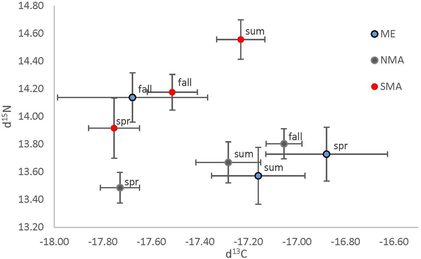
Figure 5. Mean (± 1 SE) δ13C plotted against mean (± 1 SE) δ15N, separated by region (Maine = blue, northern Massachusetts = gray and southern Massachusetts = red) and season (spring = spr, summer = sum and fall = fall).

There was a trend of higher δ¹⁵N values in SMA fish compared to those in NMA and ME. δ¹⁵N values were significantly higher for SMA fish compared to NMA fish in the spring, summer and fall (Tukey’s HSD, p < 0.05), and significantly higher than ME fish in the summer. In addition, δ¹⁵N values of ME fish were significantly higher than those of NMA fish. Finally, δ¹⁵N values for ME fish were significantly higher in the fall compared to spring and summer, for SMA fish were significantly higher in the summer compared to spring and fall, and for NMA fish were significantly higher in the fall compared to spring (Tukey’s HSD, p > 0.05 for all comparisons).

Condition

The equation W_g = 0.02 ^∗ L_t².⁸⁶ explained > 97% of the variance between length and weight of sea bass from all regions combined (Supplementary Figure S2). There was a significant interaction effect between region and season on K_rel [ANOVA, F₍₄, ₂₅₄₎ = 3.36, p = 0.01, Figure 6A]. K_rel was significantly greater for NMA and ME fish in the fall compared to the spring and summer, and significantly lower for SMA fish in the summer compared to spring and fall (Tukey’s HSD, p < 0.05 for all comparisons). K_rel was also greater for SMA fish in the spring compared to ME fish (Tukey’s HSD, p = 0.009). Mean (± 1 SE) values of K_adj (binned into 2 cm sea bass length intervals) varied greatly, but there was a decreasing trend in K_adj between 28 and 36 cm for all regions combined (Figure 7).

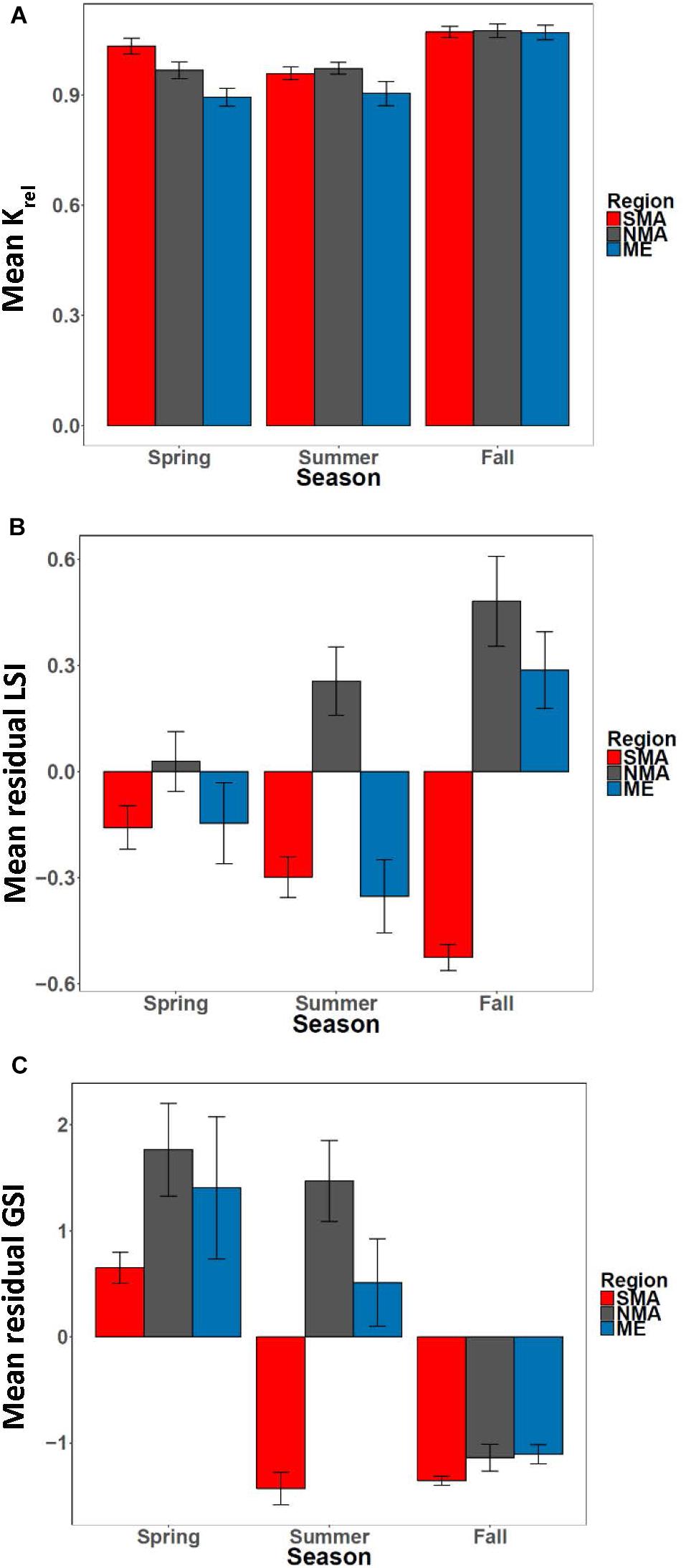
Figure 6. (A) Mean Krel, (B) mean residual LSI and (C) mean residual GSI by season for Maine (ME), northern Massachusetts (NMA) and southern Massachusetts (SMA).

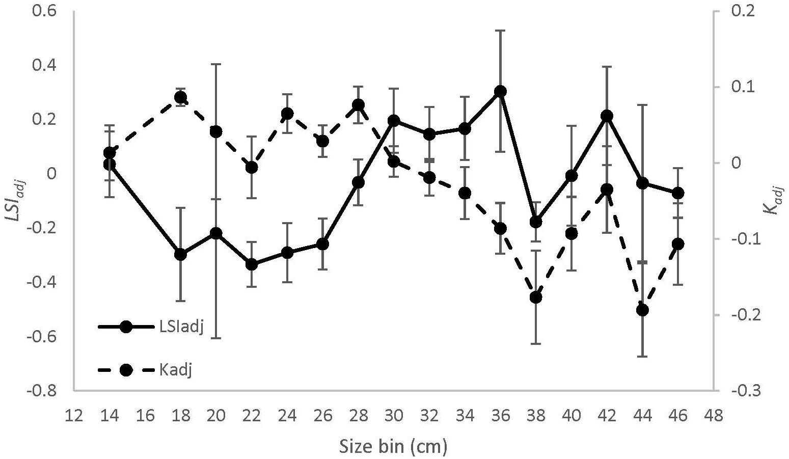
Figure 7. Mean (± 1 SE) values of Kadj (dashed line) and LSIadj (solid line) by 2 cm size bins for black sea bass from all regions combined.

There was a significant interaction between region and season [ANOVA, F₍₄, ₂₅₁₎ = 7.36, p < 0.001, Figure 6B] on residual LSI. Residual LSI was significantly lower for SMA fish in the fall compared to the spring and summer, significantly greater for ME fish in fall compared to summer, and significantly greater for NMA fish in fall compared to spring (Tukey’s HSD, p < 0.05 for all comparisons). LSI was also greater in the fall for NMA and ME fish compared to SMA fish, and greater in the summer for NMA fish compared to ME and SMA fish (Tukey’s HSD, p < 0.05 for all comparisons). Mean (± 1SE) values of LSI_adj (binned into 2 cm sea bass length intervals) also varied greatly, but contrary to K_adj results, there was a trend of increasing LSI_adj between 26 and 36 cm for all regions combined (Figure 7).

Reproduction

There was a significant interaction between region and season [ANOVA, F₍₄, ₂₄₀₎ = 7.36, p < 0.001] on residual GSI (Table 1 and Figure 6C). Residual GSI was lower for NMA and ME fish in the fall compared to spring and summer, and greater for SMA fish in the spring compared to summer and fall (Tukey’s HSD, p < 0.05 for all comparisons). Residual GSI was also lower in the spring for SMA fish compared to NMA fish, and lower in the summer for SMA fish compared to both NMA and ME fish (Tukey’s HSD, p < 0.05 for all comparisons).

There were significantly more females than males in SMA and ME (x², p < 0.05), and slightly more males than females in NMA, but this was not significant. The black sea bass sex ratio-at-length for all regions combined is shown in Figure 8A. The length at which 50% of the population was female was 33.9 cm (lower and upper 95% CI = 31.9 and 36.8 cm). Mean length at 50% maturity for all regions combined was 26.6 cm (lower and upper 95% CI = 25.6 and 27.1 cm; Figure 8B), and the age at 50% maturity for all regions combined was 1.78 (lower and upper 95% CI = 1.62 and 1.94; Figure 8C). Age-at-maturity varied among regions, with SMA having the highest age-at-maturity and NMA having the lowest. There were significantly more mature than immature sea bass collected in NMA (x², p < 0.05). The proportion of mature fish collected in SMA and ME did not differ (x², p > 0.05).

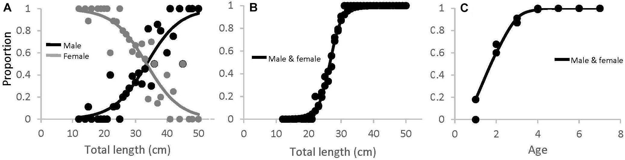
Figure 8. (A) Proportion of male (black) and female (gray) black sea bass as a function of total length for all regions combined (M₅₀ = 33.5 cm), (B) length-at-maturity (L₅₀ = 26.6 cm), and (C) age-at-maturity (A₅₀ = 1.78 years) for all regions and sexes combined.

Discussion

In the past decade, black sea bass have expanded their range into the GOM where historically cold oceans waters are now warming faster than 99% of the world’s oceans (Pershing et al., 2015), causing a shift in the distribution of suitable habitat for many species. Observations of black sea bass from SMA (i.e., historic northern range limit), NMA (i.e., newly expanded range) and ME (i.e., upper limit of newly expanded range edge), revealed variation in life-history traits across a relatively small geographic area. Significant spatial differences in size, diet, condition, maturity and sex ratio were observed. Although small sample sizes across years prevented us from analyzing inter-annual variation, which may have biased our results, our findings pooled across years suggest that range expanding sea bass may exhibit life-history strategies that differ from their southern counterparts.

Growth and Reproduction

Length-at-age estimates for all regions combined were greater than the length-at-age estimate established in the 2016 Black Sea Bass Stock Assessment, which combines length and age data from populations throughout the northern range, from Cape Hatteras to Cape Cod (Northeast Fisheries Science Center [NEFSC], 2016). We also found that sea bass from NMA and ME reach reproductive maturity at a younger age than sea bass from SMA, and that the length-at-maturity for all regions combined (L₅₀ = 26.6 cm) was greater than the length-at-maturity utilized in the most recent sea bass assessment (L₅₀ = 21 cm; Northeast Fisheries Science Center [NEFSC], 2016). These observed differences may have arisen from latitudinal variation in temperature and the length of the growing season. Organisms at higher latitudes may be locally adapted to grow within a lower range of temperatures, may have growth rates that evolve inversely with the length of the growing season (i.e., countergradient variation), or may exhibit some combination of these adaptations (Yamahira and Conover, 2002). For instance, Conover and Present (1990) found that fish from colder regions were adapted to a shorter growing season and grew faster than their southern counterparts. This effect may be due, in part, to northern fish having greater food conversion efficiencies (Present and Conover, 1992).

It is also possible that the observed differences in growth and maturity may be related to differences in migration strategies. In their native range, sea bass migrate off of the continental shelf in the winter and migrate back to nearshore habitat in the spring (Shepherd, 2008). However, very little is known about the migration patterns of sea bass in the GOM. Three potential different migration strategies could be occurring: (1) sea bass overwinter in the GOM, (2) sea bass overwinter in the Mid-Atlantic and return to the GOM each year, or (3) sea bass overwinter in the Mid-Atlantic and randomly re-occupy northern areas each year. Given the observed differences in biological metrics found in this study, it may be more likely that sea bass are overwintering in the GOM or returning to the same areas each year. Anecdotal evidence from fishers suggests that sea bass are occasionally found in offshore regions of the GOM during the winter months, further indicating that resident populations may exist. Differences in the bioenergetics of resident vs. migratory fish populations has been well documented (e.g., Forseth et al., 1999; Morinville and Rasmussen, 2003; Kerr and Secor, 2009). In particular, Morinville and Rasmussen (2003) found that resident brook trout have higher growth efficiency as a result of lower total metabolic costs. Further studies focusing on both the migration patterns and bioenergetics of sea bass in the Gulf of Maine are warranted, and may begin to uncover the mechanisms driving the latitudinal variation in growth and maturity found in this study. Furthermore, the variation in life history traits observed could have far reaching management implications as the northern stock of sea bass continues to expand poleward (Pinsky and Mantua, 2014; Hare et al., 2016; Kleisner et al., 2016, 2017).

Demographic patterns of abundance may also be influencing sea bass growth and reproduction. Range expanding sea bass populations are likely at lower densities, as evidenced by low capture rates by both fisheries dependent and independent sources, and therefore may not be subject to density-dependent competition (Burton et al., 2010; Phillips et al., 2010). These range expanding sea bass appear to be growing faster and achieving reproductive maturity at a younger age, but larger size, which follows r-K selection theory (Charlesworth, 1971; Roughgarden, 1971). Faster growth rates result in fish achieving reproductive maturity at a younger age, which promotes rapid population growth. Spatial variation in conspecific density can influence life-history traits in fish, including growth, maturation, and diet (Jones, 1987; Caselle et al., 2003, 2011; Samhouri, 2009). For example, Caselle et al. (2011) found that high density populations of California sheephead were smaller in size, had lower fecundity, and changed sex at smaller sizes, and Samhouri (2009) found that aggressive interactions in high density populations of damselfish resulted in reduced growth and reproductive output. Similar density-dependent effects may be influencing the spatial variation in black sea bass life-history traits observed among our study sites, as well as between our data and the most recent sea bass stock assessment from farther south where these effects are likely stronger (Northeast Fisheries Science Center [NEFSC], 2016).

Interspecific competition may also differ between the GOM and regions farther south. Atlantic cod, a historically dominant large bodied predator in the GOM, has rapidly decreased in abundance in recent decades, and spawning stock biomass is currently estimated to be at 5–8% of the target level (Palmer, 2017). In general, large groundfish species are functionally absent in much of the nearshore ecosystem, and have been largely replaced by smaller-bodied fish, such as sculpin and cunner (Witman and Sebens, 1992; Steneck, 1997). Sea bass are an aggressive and territorial species, and may easily outcompete small-bodied native GOM fish. For example, SCUBA and video surveys in NMA and ME have captured sea bass aggressively interacting with cunner and small pollock, generally driving them away from sea bass territories (McMahan and Grabowski, unpublished data). Therefore, in addition to potentially experiencing reduced intraspecific competition, sea bass in the GOM may also be subjected to reduced interspecific competition in comparison to those in southern regions, further minimizing the reproductive-growth trade-offs encountered in a highly competitive environment (Burton et al., 2010).

Diet and Condition

We found both regional and seasonal variability in K_rel, but overall there was a decreasing trend with latitude which may be due, in part, to variations in diet. We found that the diversity and quality of prey items in the diet of sea bass decreased with latitude. The diet of SMA sea bass was dominated by lipid rich demersal and pelagic fish, as well as squid, whereas the diet of NMA and ME sea bass was dominated by small crustaceans. Diet trends in NMA and ME were similar to results from previous studies suggesting that sea bass rely heavily on crabs and other benthic invertebrates (Mack and Bowman, 1983; Steimle and Figley, 1996; Garrison and Link, 2000). Within this study area, heterogeneity in prey availability is likely driving regional differences. For instance, many prey items found in the diet of SMA sea bass (e.g., bay anchovy, scup, squid) are rare or found in lower abundance in the GOM. However, it is unclear why SMA sea bass would consume more fish and squid than populations farther south. Stable isotope signatures reflected many of the dietary trends revealed in the stomach content analysis. ME fish had the highest δ13C values in the spring, which was also when the most shrimp and benthic invertebrate prey were found in their diet. SMA and NMA fish had higher δ13C values in the fall, which was when the greatest amount of crabs were found in their diet. δ13C values were lowest for SMA and NMA fish in the spring, however, this was also the period of time when very few fish and squid were found in their diet. Therefore, there may be a prey source that these fish consume in the spring (i.e., when sea bass are migrating from the continental shelf to nearshore spawning habitat) that was not found in stomach content results.

Ontogenetic trends in diet revealed that feeding habits also fluctuated with fish size and that Kadj closely tracked diet trends. We were unable to compare ontogenetic trends in diet and condition among regions due to low sample sizes. However, in general, we found that fish between 28 and 36 cm total length decreased their feeding and shifted from consuming predominantly squid and fish to crabs, which coincided with a decrease in their K_adj. Sherwood et al. (2002) found that prey switching often occurs when condition starts to decline, suggesting that these diet changes may be necessary to overcome energetic bottlenecks. Yet, counterintuitively, LSI_adj increased within this size range, suggesting that further research will likely be needed to resolve whether it is an energetic bottleneck. It is also possible that the allocation of energy shifts during certain growth phases, causing liver and somatic condition to diverge. As individuals allocate energy to fat reserves (i.e., lipid storage in the liver) they must reduce energy allocation to somatic growth. Therefore, sea bass storing energy for periods without feeding, such as spawning, may exhibit decreased somatic growth and increased lipid storage.

The range of LSI and GSI values obtained in this study were similar to values previously reported for sea bass collected in SMA (Wuenschel et al., 2013). LSI varied among season, but was highest in the fall for NMA and ME, and was inversely correlated with GSI. This finding may indicate that sea bass in the GOM are using energy reserves in the liver while spawning, and that those reserves are replenished when spawning concludes in the late summer and fall. It is also possible that this energy allocation strategy relates to the fall migration of sea bass in the GOM, however, very little is known about seasonal movement patterns of sea bass in this newly expanded region. The opposite energy allocation trend was found in SMA. LSI decreased from spring to fall and was positively correlated with GSI. LSI values in SMA were also lower than in NMA and ME. We speculate that this could have been related to increased consumption of fish and squid in SMA. As spawning decreased from spring to fall for SMA fish, consumption may have rapidly increased. A substantial increase in body weight would sharply increase the denominator of the LSI equation, leading to decreased LSI values (Brown and Murphy, 2004). Overall, these results suggest that sea bass in SMA may exhibit different energetic strategies than sea bass in the GOM, and that parameters from sea bass caught within the historic range may not accurately predict the biology and population dynamics of sea bass in the GOM. Further investigation of how energetic strategies vary with latitude is warranted.

Regional differences in GSI may reflect a latitudinal gradient in the length of the spawning season. Sea bass in SMA are likely able to spawn earlier in the spring due to warmer temperatures and a shorter migration from offshore winter habitat. We collected sea bass between mid-May and mid-June in the spring season. In SMA, GSI may have already begun to decrease during this period if spawning began earlier than mid-May. Conversely, GSI was much higher in NMA and ME during the spring, perhaps because spawning is delayed at higher latitudes. In the summer season, GSI was greatly reduced in SMA as spawning was likely ending, and GSI values were similarly low among all regions in the fall.

Size and Sex Ratio

We found that the sex ratio of all regions combined was 100% female for the smallest sizes and approached 100% male for the largest sizes. This pattern is typical of a hermaphroditic species that matures as a female and transitions to male as it grows, however, our results were markedly different from previous black sea bass work that has found sex ratios of approximately 30% male below 30 cm, and 30–40% female above 45 cm (Wuenschel et al., 2011; Northeast Fisheries Science Center [NEFSC], 2012, 2016; Blaylock and Shepherd, 2016). Indeed, the northern stock of black sea bass in its historic range is distinguished from typical protogynous hermaphrodites because of the presence of secondary mature males and the abundance of large females in their population (Blaylock and Shepherd, 2016). Blaylock and Shepherd (2016) concluded that black sea bass are likely more resilient to fisheries exploitation because of these unique sex ratios. Our results did not reveal a similar abundance of smaller males and larger females, which may be a consequence of small sample sizes of the smallest and largest black sea bass size categories. We analyzed a total of 288 sea bass, whereas the stock assessment utilizes results from thousands of sea bass throughout the northern range (but south of Cape Cod). However, it is also possible that range expanding populations do not reflect the same sex-ratio trends as populations near the center of their range.

In addition, we found that sex ratios varied with region, with 20–30% males and 70–80% females in SMA and ME, and 55% males and 45% females in NMA. We also found that sea bass were larger in NMA and predominantly mature. Caruso (1995) observed that the majority of sea bass recruiting to SMA where mature, and at the time of these observations (early 1990s), SMA was considered the range edge of the northern stock. These results indicate that sea bass populations have shifted, and that large, mature fish are now recruiting to NMA. Meanwhile, small, immature fish (i.e., those that can be outcompeted by larger fish) are common farther north in ME, where conspecific density is lower, but habitat may be suboptimal (i.e., colder temperature and less diverse prey availability).

Conclusion

Collectively, these results suggest that demographic patterns and life-history strategies of range expanding sea bass differ from more centralized populations, and that important stock metrics, such as growth and maturity, vary over relatively short distances. Previous black sea bass stock assessment reviews explicitly called for the incorporation of spatial structure within the northern stock due to concern that incomplete mixing was occurring (Northeast Fisheries Science Center [NEFSC], 2016). In response, the most recent sea bass stock assessment incorporated a spatial divide at the Hudson Canyon and found that the two-area model better represented overall population dynamics (Northeast Fisheries Science Center [NEFSC], 2016). However, our results suggest that latitudinal heterogeneity exists in sea bass populations north of the Hudson Canyon divide. Furthermore, the poleward range expansion of black sea bass is predicted to continue as additional warming occurs along the U.S. Northeast Continental Shelf (Kleisner et al., 2016, 2017), which could result in further divergence of life-history traits of range expanding sea bass away from more centralized populations. We recommend that future assessments target GOM sea bass to build upon these initial findings and enhance our understanding of the biology and population dynamics of sea bass in their newly expanded range. Finally, these findings apply more broadly to the global redistribution of species that is currently underway and expected to intensify (Pecl et al., 2017), and emphasize the need to incorporate alternative assessment and management approaches to range shifting species.

Data Availability Statement

All datasets presented in this study are included in the article/Supplementary Material.

Ethics Statement

Ethical review and approval was not required for this animal study as samples were obtained by fishermen or state/federal agencies (Maine Department of Marine Resource, Massachusetts Division of Marine Fisheries, and the Northeast Fisheries Science Center).

Author Contributions

MM and JG designed and carried out the research. MM conducted the analyses. MM, JG, and GS contributed to writing and reviewing the manuscript. All authors contributed to the article and approved the submitted version.

Funding

Funding for this project was provided by the Graduate Women in Science Nell Mondy Fellowship, the Switzer Environmental Fellowship, crowd funding sourced through Experiment, and the NOAA Saltonstall-Kennedy Grant Program: Award # NA18NMF4270189.

Conflict of Interest

The authors declare that the research was conducted in the absence of any commercial or financial relationships that could be construed as a potential conflict of interest.

Acknowledgments

We thank the Massachusetts Division of Marine Fisheries, Maine Department of Marine Resources, Kevin Cheung, William Lister, Jim McMahan, and Richard Nelson for collecting sea bass. We also thank R. Waller, S. Elzey, K. O’Brien, K. Schultz, A. Scrippa, and C. Lawrence for assistance in the laboratory. Finally, this manuscript was greatly improved thanks to comments and edits provided by three reviewers.

Supplementary Material

The Supplementary Material for this article can be found online at: https://www.frontiersin.org/articles/10.3389/fmars.2020.567758/full#supplementary-material

References

Alonzo, S. H., Ish, T., Key, M., MacCall, A. D., and Mangel, M. (2008). The importance of incorporating protogynous sex change into stock assessments. Bull. Mar. Sci. 83, 163–179.
Bell, R. J., Richardson, D. E., Hare, J. A., Lynch, P. D., and Fratantoni, P. S. (2015). Disentangling the effects of climate, abundance, and size on the distribution of marine fish: an example based on four stocks from the Northeast US shelf. ICES J. Mar. Sci. 72, 1311–1322. doi: 10.1093/icesjms/fsu217
Benard, M. F. (2004). Predator-induced phenotypic plasticity in organisms with complex life histories. Annu. Rev. Ecol. Evol. Syst. 35, 651–673. doi: 10.1146/annurev.ecolsys.35.021004.112426
Blaylock, J., and Shepherd, G. R. (2016). Evaluating the vulnerability of an atypical protogynous hermaphrodite to fishery exploitation: results from a population model for black sea bass (Centropristis striata). Fishery Bull. 114, 476–489. doi: 10.7755/FB.114.4.9
Bowering, W. R., and Lilly, G. R. (1992). Greenland halibut (Reinhardtius hippoglossoides) off southern Labrador and northeastern Newfoundland (Northwest Atlantic) feed primarily on capelin (Mallotus villosus). Neth. J. Sea Res. 29, 211–222. doi: 10.1016/0077-7579(92)90021-6
Brander, K. (2010). Impacts of climate change on fisheries. J. Mar. Syst. 79, 389–402. doi: 10.1016/j.jmarsys.2008.12.015
Bretz, F., Hothorn, T., and Westfall, P. (2010). Multiple Comparisons Using R. Boca Raton, FL: CRC Press.
Brown, M. L., and Murphy, B. R. (2004). Seasonal dynamics of direct and indirect condition indices in relation to energy allocation in largemouth bass Micropterus salmoides (Lacepede). Ecol. Freshw. Fish 13, 23–36. doi: 10.1111/j.0906-6691.2004.00031.x
Buchheister, A., and Latour, R. J. (2015). Dynamic trophic linkages in a large estuarine system—support for supply-driven dietary changes using delta generalized additive mixed models. Can. J. Fish. Aquat. Sci. 73, 5–17. doi: 10.1139/cjfas-2014-0441
Burton, O. J., Phillips, B. L., and Travis, J. M. (2010). Trade-offs and the evolution of life-histories during range expansion. Ecol. Lett. 13, 1210–1220. doi: 10.1111/j.1461-0248.2010.01505.x
Cadrin, S. X., and Secor, D. H. (2009). “Accounting for spatial population structure in stock assessment: past, present, and future,” in The Future of Fisheries Science in North America, eds R. J. Beamish and B. J. Rothschild (Dordrecht: Springer), 405–426. doi: 10.1007/978-1-4020-9210-7_22
Caruso, P. G. (1995). The Age, Growth, and Spawning of Black Sea Bass (Centropristis striata, Linneaus) in Massachusetts Waters. Master’s thesis, University of Rhode Island, Kingston, RI, 117.
Caselle, J. E., Hamilton, S. L., Schroeder, D. M., Love, M. S., Standish, J. D., Rosales-Casian, J. A., et al. (2011). Geographic variation in density, demography, and life history traits of a harvested, sex-changing, temperate reef fish. Can. J. Fish. Aquat. Sci. 68, 288–303. doi: 10.1139/F10-140
Caselle, J. E., Hamilton, S. L., and Warner, R. R. (2003). The interaction of retention, recruitment, and density-dependent mortality in the spatial placement of marine reserves. Gulf Caribbean Res. 14, 107–116. doi: 10.18785/gcr.1402.08
Charlesworth, B. (1971). Selection in density-regulated populations. Ecology 52, 469–474. doi: 10.2307/1937629
Ciannelli, L., Fauchald, P., Chan, K. S., Agostini, V. N., and Dingsør, G. E. (2008). Spatial fisheries ecology: recent progress and future prospects. J. Mar. Syst. 71, 223–236. doi: 10.1016/j.jmarsys.2007.02.031
Conover, D. O. (1990). The relation between capacity for growth and length of growing season: evidence for and implications of countergradient variation. Trans. Am. Fish. Soc. 119, 416–430. doi: 10.1577/1548-8659(1990)119<0416:TRBCFG>2.3.CO;2
Conover, D. O., and Present, T. M. (1990). Countergradient variation in growth rate: compensation for length of the growing season among Atlantic silversides from different latitudes. Oecologia 83, 316–324. doi: 10.1007/BF00317554
Drohan, A. F., Manderson, J. P., and Packer, D. B. (2007). Essential Fish Habitat Source Document: Black Sea Bass, Centropristis striata, Life History and Habitat Characteristics, 2nd Edn. Available online at: http://www.nefsc.noaa.gov/nefsc/publications/tm/tm200/ (accessed September, 2014).
Elzey, S. P., Trull, K. J., and Rogers, K. A. (2015). Massachusetts Division of Marine Fisheries Age and Growth Laboratory: Fish Aging Protocols. Gloucester, MA: Massachusetts Division of Marine Fisheries.
Forseth, T., Naesje, T. F., Jonsson, B., and Harsåker, K. (1999). Juvenile migration in brown trout: a consequence of energetic state. J. Anim. Ecol. 68, 783–793. doi: 10.1046/j.1365-2656.1999.00329.x
Froese, R. (2006). Cube law, condition factor and Length-Weight relationships: history, meta-analysis and recommendations. Appl. Ichthyol. 22, 241–253. doi: 10.1111/j.1439-0426.2006.00805.x
Fry, B. (1988). Food web structure on Georges Bank from stable C, N, and S isotopic compositions. Limnol. Oceanogr. 33, 1182–1190. doi: 10.4319/lo.1988.33.5.1182
Garrison, L. P., and Link, J. S. (2000). Dietary guild structure of the fish community in the Northeast United States continental shelf ecosystem. Mar. Ecol. Prog. Ser. 202, 231–240. doi: 10.3354/meps202231
Gower, J. C. (1971). A general coefficient of similarity and some of its properties. Biometrics 27, 857–874. doi: 10.2307/2528823
Hare, J. A., Morrison, W. E., Nelson, M. W., Stachura, M. M., Teeters, E. J., Griffis, R. B., et al. (2016). A vulnerability assessment of fish and invertebrates to climate change on the Northeast US Continental Shelf. PLoS One 11:e0146756. doi: 10.1371/journal.pone.0146756
Hothorn, T., Bretz, F., and Westfall, P. (2008). Simultaneous inference in general parametric models. Biom. J. 50, 346–363. doi: 10.1002/bimj.200810425
Jones, G. P. (1987). Competitive interactions among adults and juveniles of a coral reef fish. Ecology 68, 1534–1547. doi: 10.2307/1939237
Jorgensen, C., Enberg, K., Dunlop, E. S., Arlinghaus, R., Boukal, D. S., Brander, K., et al. (2007). Ecology-Managing evolving fish stocks. Science 318, 1247–1248. doi: 10.1126/science.1148089
Kerr, L. A., and Secor, D. H. (2009). Bioenergetic trajectories underlying partial migration in Patuxent River (Chesapeake Bay) white perch (Morone americana). Can. J. Fish. Aquat. Sci. 66, 602–612. doi: 10.1139/F09-027
Kleisner, K. M., Fogarty, M. J., McGee, S., Barnett, A., Fratantoni, P., Greene, J., et al. (2016). The effects of sub-regional climate velocity on the distribution and spatial extent of marine species assemblages. PLoS One 11:e0149220. doi: 10.1371/journal.pone.0149220
Kleisner, K. M., Fogarty, M. J., McGee, S., Hare, J. A., Moret, S., Perretti, C. T., et al. (2017). Marine species distribution shifts on the US Northeast Continental Shelf under continued ocean warming. Prog. Oceanogr. 153, 24–36. doi: 10.1016/j.pocean.2017.04.001
Kolek, D. (1990). Homing of Black Sea Bass, Centropristis striata, in Nantucket Sound with Comments on Seasonal Distribution, Growth Rates, and Fisheries of the Species. Boston, MA: Massachusetts Division of Marine Fisheries, 12.
Lawing, A. M., and Polly, P. D. (2011). Pleistocene climate, phenology, and climate envelope models: an integrative approach to better understand species’ response to climate change. PLoS One 6:e28554. doi: 10.1371/journal.pone.0028554
Le Cren, E. D. (1951). The length-weight relationships and seasonal cycle in gonad weight and condition in the perch (Perca fluviatilis). J. Anim. Ecol. 20, 201–219.
Link, J. S., Nye, J. A., and Hare, J. A. (2011). Guidelines for incorporating fish distribution shifts into a fisheries management context. Fish Fish. 12, 461–469.
Lorenzen, K., Steneck, R. S., Warner, R. R., Parma, A. M., Coleman, F. C., and Leber, K. M. (2010). The spatial dimensions of fisheries: putting it all in place. Bull. Mar. Sci. 86, 169–177.
Mack, R. G. Jr., and Bowman, R. E. (1983). Food and Feeding of Black Sea Bass (Centropristis striata). Woods Hole Laboratory Reference Document. Woods Hole, MA: Northeast Fisheries Center.
McCartney, M. A., Burton, M. L., and Lima, T. G. (2013). Mitochondrial DNA differentiation between populations of black sea bass (Centropristis striata) across Cape Hatteras, North Carolina (USA). J. Biogeogr. 40, 1386–1398.
McGovern, J. C., Collins, M. R., Pashuk, O., and Meister, H. S. (2002). Temporal and spatial differences in life history parameters of black sea bass in the southeastern United States. North Am. J. Fish. Manage. 22, 1151–1163.
Morinville, G. R., and Rasmussen, J. B. (2003). Early juvenile bioenergetic differences between anadromous and resident brook trout (Salvelinus fontinalis Can. J. Fish. Aquat. Sci. 60, 401–410. doi: 10.1139/F03-036
Moser, J., and Shepherd, G. R. (2009). Seasonal distribution and movement of black sea bass (Centropristis striata) in the Northwest Atlantic as determined from a mark-recapture experiment. J. Northwest Atl. Fishery Sci. 40, 17–28.
Northeast Fisheries Science Center [NEFSC] (2012). 53rd Northeast Regional Stock Assessment Workshop (53rd SAW) Assessment Report. US Department of Commerce, Northeast Fisheries Science Center Reference Document. Woods Hole, MA: National Marine Fisheries Service.
Northeast Fisheries Science Center [NEFSC] (2016). 62nd Northeast Regional Stock Assessment Workshop (62nd SAW) Assessment Report. US Department of Commerce, Northeast Fisheries Science Center Reference Document. Woods Hole, MA: National Marine Fisheries Service.
Ogle, D. H., Wheeler, P., and Dinno, A. (2020). FSA: Fisheries Stock Analysis. R package version 0.8.30.9000. Available online at: https://github.com/droglenc/FSA (accessed July 6, 2020).
Owens, N. J. P. (1987). Natural variation in 15N in the marine environment. Adv. Mar. Biol. 24, 389–450. doi: 10.1016/S0065-2881(08)60077-2
Palmer, M. (2017). Gulf of Maine Atlantic Cod 2017 Assessment Update Report. Woods Hole, MA: National Marine Fisheries Service.
Parmesan, C., and Yohe, G. (2003). A globally coherent fingerprint of climate change impacts across natural systems. Nature 421, 37–42. doi: 10.1038/nature01286
Pascoe, S., Bustamante, R., Wilcox, C., and Gibbs, M. (2009). Spatial fisheries management: a framework for multi-objective qualitative assessment. Ocean Coast. Manage. 52, 130–138. doi: 10.1016/j.ocecoaman.2008.10.009
Pauly, D. (1980). On the interrelationships between natural mortality, growth parameters, and mean environmental temperature in 175 fish stocks. ICES J. Mar. Sci. 39, 175–192. doi: 10.1093/icesjms/39.2.175
Pecl, G. T., Araújo, M. B., Bell, J. D., Blanchard, J., Bonebrake, T. C., Chen, I. C., et al. (2017). Biodiversity redistribution under climate change: impacts on ecosystems and human well-being. Science 355:eaai9214. doi: 10.1126/science.aai9214
Perry, A. L., Low, P. J., Ellis, J. R., and Reynolds, J. D. (2005). Climate change and distribution shifts in marine fishes. Science 308, 1912–1915. doi: 10.1126/science.1111322
Pershing, A. J., Alexander, M. A., Hernandez, C. M., Kerr, L. A., Le Bris, A., Mills, K. E., et al. (2015). Slow adaptation in the face of rapid warming leads to collapse of the Gulf of Maine cod fishery. Science 350, 809–812. doi: 10.1126/science.aac9819
Phillips, B. L., Brown, G. P., and Shine, R. (2010). Life-history evolution in range-shifting populations. Ecology 91, 1617–1627. doi: 10.1890/09-0910.1
Pinsky, M. L., and Mantua, N. J. (2014). Emerging adaptation approaches for climate-ready fisheries management. Oceanography 27, 146–159. doi: 10.5670/oceanog.2014.93
Poloczanska, E. S., Brown, C. J., Sydeman, W. J., Kiessling, W., Schoeman, D. S., Moore, P. J., et al. (2013). Global imprint of climate change on marine life. Nat. Clim. Change 3, 919–925. doi: 10.1038/nclimate1958
Pörtner, H. O., Berdal, B., Blust, R., Brix, O., Colosimo, A., De Wachter, B., et al. (2001). Climate induced temperature effects on growth performance, fecundity and recruitment in marine fish: developing a hypothesis for cause and effect relationships in Atlantic cod (Gadus morhua) and common eelpout (Zoarces viviparus). Cont. Shelf Res. 21, 1975–1997. doi: 10.1016/S0278-4343(01)00038-3
Present, T. M. C., and Conover, D. O. (1992). Physiological basis of latitudinal growth differences in Menidia menidia: variation in consumption or efficiency? Funct. Ecol. 6, 23–31. doi: 10.2307/2389767
Provost, M. M., and Jensen, O. P. (2015). The impacts of fishing on hermaphroditic and treatment of sex change in stock assessments. Fisheries 40, 536–545. doi: 10.1080/03632415.2015.1093471
R Core Team (2017). R: A Language and Environment for Statistical Computing. Vienna: R Foundation for Statistical Computing.
Reznick, D. A., Bryga, H., and Endler, J. A. (1990). Experimentally induced life-history evolution in a natural population. Nature 346, 357–359. doi: 10.1038/346357a0
Robillard, E., Gregg, J. W., Dayton, J., and Gartland, J. (2011). Validation of Black Sea Bass, Centropristis striata, Ages Using Oxytetracycline Marking and Scale Margin Increments. SARC 62 Working Paper. Woods Hole, MA: Northeast Fisheries Science Center.
Roff D. (ed.) (1993). Evolution of Life. (Histories): Theory and Analysis. New York, NY: Chapman and Hall.
Roughgarden, J. (1971). Density-dependent natural selection. Ecology 52, 453–468. doi: 10.2307/1937628
Sagarin, R. D., and Gaines, S. D. (2002). The ‘abundant center’ distribution: to what extent is it a biogeographical rule? Ecol. Lett. 5, 137–147. doi: 10.1046/j.1461-0248.2002.00297.x
Samhouri, J. F. (2009). Food supply influences offspring provisioning but not density-dependent fecundity in a marine fish. Ecology 90, 3478–3488. doi: 10.1890/08-1732.1
Santos, M., German, I., Correia, D., Read, F., Martinez Cedeira, J., Caldas, M., et al. (2013). Long-term variation in common dolphin diet in relation to prey abundance. Mar. Ecol. Prog. Ser. 481, 249–268. doi: 10.3354/meps10233
Shepherd, G. R. (2008). Black Sea Bass. The Northeast Data Poor Stocks Working Group Report. Available online at: file:///C:/Users/ELCOT/Downloads/NEFSC_RD_09_02.pdf (accessed November 24, 2017).
Sherwood, G. D., Pazzia, I., Moeser, A., Hontela, A., and Rasmussen, J. B. (2002). Shifting gears: enzymatic evidence for the energetic advantage of switching diet in wild-living fish. Can. J. Fish. Aquat. Sci. 59, 229–241. doi: 10.1139/f02-001
Sherwood, G. D., Rideout, R. M., Fudge, S. B., and Rose, G. A. (2007). Influence of diet on growth, condition and reproductive capacity in Newfoundland and Labrador cod (Gadus morhua): insights from stable carbon isotopes (δ 13 C). Deep Sea Res Part II Top. Stud. Oceanogr. 54, 2794–2809. doi: 10.1016/j.dsr2.2007.08.007
Sherwood, G. D., and Rose, G. A. (2005). Stable isotope analysis of some representative fish and invertebrates of the Newfoundland and Labrador continental shelf food web. Estuar. Coast. Shelf Sci. 63, 537–549. doi: 10.1016/j.ecss.2004.12.010
Stefánsson, G. (1996). Analysis of groundfish survey abundance data: combining the GLM and delta approaches. ICES J. Mar. Sci. 53, 577–588. doi: 10.1006/jmsc.1996.0079
Stefánsson, G., and Pálsson, Ó. K. (1997). Statistical evaluation and modelling of the stomach contents of Icelandic cod (Gadus morhua). Can. J. Fish. Aquat. Sci. 54, 169–181. doi: 10.1139/f96-246
Steimle, F. W., and Figley, W. (1996). The importance of artificial reef epifauna to black sea bass diets in the Middle Atlantic Bight. North Am. J. Fish. Manage. 16, 433–439. doi: 10.1577/1548-8675(1996)016<0433:TIOARE>2.3.CO;2
Steneck, R. S. (1997). “Fisheries-induced biological changes to the structure and function of the Gulf of Maine ecosystem,” in Proceedings of the Gulf of Maine Ecosystem Dynamics Scientific Symposium and Workshop. RARGOM Report, eds G. T. Wallace and E. F. Braasch (Hanover, NH: Regional Association for Research on the Gulf of Maine), 151–165.
Witman, J. D., and Sebens, K. P. (1992). Regional variation in fish predation intensity: a historical perspective in the Gulf of Maine. Oecologia 90, 305–315. doi: 10.1007/BF00317686
Wuenschel, M. J., McBride, R. S., and Fitzhugh, G. R. (2013). Relations between total gonad energy and physiological measures of condition in the period leading up to spawning: results of a laboratory experiment on black sea bass (Centropristis striata). Fish. Res. 138, 110–119. doi: 10.1016/j.fishres.2012.05.012
Wuenschel, M. J., Shepherd, G. R., McBride, R. S., Jorgensen, R., Oliveira, K., Robillard, E., et al. (2011). Sex and Maturity Of Black Sea Bass Collected in Massachusetts and Rhode Island Waters; Preliminary Results Based on Macroscopic Staging of Gonads with a Comparison to Survey Data. Silver Spring, MD: National Oceanic and Atmospheric Administration.
Yamahira, K., and Conover, D. O. (2002). Intra- vs interspecific latitudinal variation in growth: adaptation to temperature or seasonality? Ecology 83, 1252–1262. doi: 10.1890/0012-9658(2002)083[1252:IVILVI]2.0.CO;2
Keywords: black sea bass, range expansion, life-history traits, warming water, Gulf of Maine, population dynamics
Citation: McMahan MD, Sherwood GD and Grabowski JH (2020) Geographic Variation in Life-History Traits of Black Sea Bass (Centropristis striata) During a Rapid Range Expansion. Front. Mar. Sci. 7:567758. doi: 10.3389/fmars.2020.567758
Received: 30 May 2020; Accepted: 02 September 2020;
Published: 25 September 2020.
Edited by:
Paul E. Renaud, Akvaplan niva, NorwayReviewed by:
Jonathan Arthur Hare, Northeast Fisheries Science Center (NOAA), United StatesKhor Waiho, University of Malaysia Terengganu, Malaysia
Sybrand Alexander Hesp, Department of Primary Industries and Regional Development of Western Australia (DPIRD), Australia
Copyright © 2020 McMahan, Sherwood and Grabowski. This is an open-access article distributed under the terms of the Creative Commons Attribution License (CC BY). The use, distribution or reproduction in other forums is permitted, provided the original author(s) and the copyright owner(s) are credited and that the original publication in this journal is cited, in accordance with accepted academic practice. No use, distribution or reproduction is permitted which does not comply with these terms.
*Correspondence: Marissa D. McMahan, mmcmahan@manomet.org